A quick guide to automated remote sensing analyses.
Spirit Mound is a prominent landform protruding a little over 100 ft above the surrounding glacial till covered plains. Geologically, it is a remnant of resistant Niobrara Chalk that survived numerous glacial advances during the Ice Age. Ecologically, the mound and surrounding area are actively being restored back to a natural prairie, creating habitat for many plants, birds, and insects.
Spirit Mound also has a history with the Native Americans that once inhabited the area. The Omaha, the Sioux, and the Otoes tribes believed that the mound was occupied by spirits that killed any human who came near. The famous explorers Lewis and Clark became aware of this legend and visited the mound 1804 to see for themselves. They reported seeing many buffalo and other wildlife from atop the mound but not much in the way of spirits. In 1986 the Spirit Mound Trust was formed to restore the mound and the surrounding 360 acres to its natural prairie state for future generations admire. If you want to know more about Spirit Mound visit www.spiritmound.org.
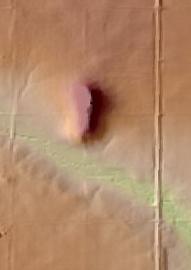
This year in April a fire broke out and burned about 100 acres. The fire was caused by a rouge spark from another fire at a nearby farm. Thankfully nobody was hurt, although some of the buildings suffered damage. Fortunately, fire is very good for prairies and a controlled burn was planned for this year anyway.
I serve on the board of directors for the Spirit Mound Trust, so I wanted to do some remote sensing analyses to get the geometry of the burn site and provide a brief tutorial on how to do so.
To do this I used Landsat 8 Imagery and looked at the Normalized Vegetation Index (NDVI), Normalized Burn Ratio (NBR), and regular RGB images.
NDVI and NBR
NDVI is basically a measurement of how green the land surface is. It is calculated from the near-infrared (NIR) and red bands of satellite imagery with the following equation:
NDVI = (NIR-Red)/(NIR+Red)
Healthy plants absorb most of the visible light spectrum and reflects a large amount of NIR portion of the electromagnetic spectrum (EMS). Unhealthy vegetation or sparsely vegetated areas reflect more visible light and less NIR.
NBR is similar to NDVI but instead of the red band it is uses the shortwave-infrared (SWIR) band of satellite imagery with the following equation:
NBR = (NIR-SWIR)/(NIR+SWIR)
Plants reflect strongly in the NIR portion of the EMS but much less strongly in the SWIR portion of the EMS. Conversely, NIR reflects much less and SWIR much more where burned wood, soil, and earth are, making this index a very powerful way to assess fire scars.
Analysis
I did the analysis in a Jupyter Notebook, which you can download here: https://github.com/nlamkey/Spirit-Mound-Fire.
First you need to find Landsat imagery to analyze and then you’ll need to set up the dependencies, directories and paths to the data.
import os
from glob import glob
import warnings

import matplotlib.pyplot as plt
import numpy as np
import geopandas as gpd
import pandas as pd
import rioxarray as rxr
import xarray as xr
import rasterio as rio
from rasterio.plot import plotting_extent

import earthpy.spatial as es
import earthpy.plot as ep
import earthpy as et
import pyproj
import fiona

pyproj.set_use_global_context(True)


# Paths to data

path_to_drive = os.path.join("D:\\")
working_dir = os.path.join(path_to_drive, 'SpiritMound')

site_boundary_path = os.path.join(working_dir,
                                  'shapefiles',
                                  'spiritmound_boundary.shp')

test_data_path = os.path.join(working_dir,
                              "tar",
                              "LC08_L2SP_029030_20220315_20220322_02_T1",
                              "LC08_L2SP_029030_20220315_20220322_02_T1_SR_B4.tif")

all_data_path = os.path.join(working_dir,
                             "tar")
Next, define some functions that are useful for getting raster stats and masking any Landsat imagery with clouds. The masking functions allow you to use the pixel qa layer of Landsat imagery to remove any values you supply to the function variable vals. You can get these numbers from the Data Format Control Book for the dataset you’re working with.
def print_raster(raster):
    print(
        f"shape: {raster.rio.shape}\n"
        f"resolution: {raster.rio.resolution()}\n"
        f"bounds: {raster.rio.bounds()}\n"
        f"sum: {raster.sum().item()}\n"
        f"CRS: {raster.rio.crs}\n"
    )

def open_clean_bands(band_path,
                     site_bound,
                     variable=None,
                     valid_range=None,
                     ):

    band = rxr.open_rasterio(band_path,
                             masked=True,
                             variable=variable,
                             from_disk=True).rio.clip(geometries=site_bound,from_disk=True).squeeze()

    if valid_range:
        mask = ((band < valid_range[0]) | (band > valid_range[1]))
        band = band.where(~xr.where(mask, True, False))

    return band

def mask_ndvi(all_bands,
              vals,
              raster):
    """Open and mask a single landsat band using a pixel_qa layer.

    Parameters
    -----------
    all_bands : list
        A list containing two xarray objects for landsat bands 4 and  5
    vals: list
        A list of values needed to create the cloud mask


    Returns
    -----------
    ndvi_mask : Xarray Dataset
        a masked xarray object containing NDVI values
    """

    # Calculate NDVI
    ndvi_xr = (all_bands[1]-all_bands[0]) / (all_bands[1]+all_bands[0])

    # Apply cloud mask to NDVI
    ndvi_mask = ndvi_xr.where(~raster.isin(vals))

    return ndvi_mask

def mask_nbr(all_bands,
              vals,
              raster):
    """Open and mask a single landsat band using a pixel_qa layer.

    Parameters
    -----------
    all_bands : list
        A list containing two xarray objects for landsat bands 5 and  7
    vals: list
        A list of values needed to create the cloud mask


    Returns
    -----------
    nbr_mask : Xarray Dataset
        a masked xarray object containing NDVI values
    """

    # Calculate NBR
    nbr_xr = (all_bands[1]-all_bands[3]) / (all_bands[1]+all_bands[3])

    # Apply cloud mask to NDVI
    nbr_mask = nbr_xr.where(~raster.isin(vals))

    return nbr_mask
Get a list of all the folders that contain the Landsat data using glob.
In: dirs = glob(all_data_path + "/*/")Out: ['D:\\SpiritMound\\tar\\LC08_L2SP_029030_20220315_20220322_02_T1\\',
'D:\\SpiritMound\\tar\\LC08_L2SP_029030_20220416_20220420_02_T1\\',
'D:\\SpiritMound\\tar\\LC08_L2SP_029030_20220518_20220525_02_T1\\',
'D:\\SpiritMound\\tar\\LC09_L2SP_029030_20220408_20220520_02_T1\\']Set up a loop to automate the process of calculating NDVI. This loop opens up the necessary bands for the NDVI calculation in an xarray dataset, clips the data to a project extent, and masks any clouds with NA values. It also writes the data out to the disk so be ready for that.
# Open and process NDVI data
vals = [22280,
        24088, 24216, 24344, 24472, 55052, 56856, 56984, 57240]
ndvi_list=[]
date_list=[]
ndvi_plot=[]
for i in dirs:
    band_paths = sorted(glob(os.path.join(i, "*B*[4-5].tif")))

    pixel_qa_path = sorted(glob(os.path.join(i, "*QA_PIXEL*")))

    folder_name = os.path.basename(os.path.normpath(i))
    data_type_name = folder_name[0:4]
    date = folder_name[17:25]
    date_list.append(date)
    mean_ndvi_df = pd.DataFrame()
    out_xr = []
    out_pixel = []
    for band, tif_path in enumerate(band_paths):

        out_xr.append(open_clean_bands(band_path=tif_path,
                                       valid_range=(7273,43636),
                                       site_bound=shapes))

        out_xr[band]["band"] = band+1

    xr.concat(out_xr, dim="band")

    for k in pixel_qa_path:
        pixel_qa = rxr.open_rasterio(k, masked=True).rio.clip(geometries=shapes,
                                                                      from_disk=True).squeeze()
        ndvi = mask_ndvi(all_bands=out_xr,
                         vals=vals,
                         raster=pixel_qa)

        file_name = data_type_name + date + '.tif'
        out_path = os.path.join(output_dir, file_name)

        ndvi_clip = ndvi.rio.clip(geometries=shapes,
                                  all_touched=True,
                                  from_disk=True).squeeze()
        mean_ndvi=np.nanmean(ndvi_clip)
        ndvi_list.append(mean_ndvi)
        mean_ndvi_df["date"] = date_list
        mean_ndvi_df['mean_ndvi'] = ndvi_list

        ndvi_plot.append(ndvi_clip)
        ndvi_clip.rio.to_raster(out_path)
The same loop but different bands for NBR.
# Open process NBR data
vals = [22280,
        24088, 24216, 24344, 24472, 55052, 56856, 56984, 57240]
nbr_list=[]
date_list=[]
nbr_plot=[]
for i in dirs:
    band_paths = sorted(glob(os.path.join(i, "*B*[4-7].tif")))

    pixel_qa_path = sorted(glob(os.path.join(i, "*QA_PIXEL*")))

    folder_name = os.path.basename(os.path.normpath(i))
    data_type_name = folder_name[0:4]
    date = folder_name[17:25]
    date_list.append(date)
    mean_nbr_df = pd.DataFrame()
    out_xr = []
    out_pixel = []
    for band, tif_path in enumerate(band_paths):

        out_xr.append(open_clean_bands(band_path=tif_path,
                                       valid_range=(7273,43636),
                                       site_bound=shapes))

        out_xr[band]["band"] = band+1

    xr.concat(out_xr, dim="band")

    for k in pixel_qa_path:
        pixel_qa = rxr.open_rasterio(k, masked=True).rio.clip(geometries=shapes,
                                                                      from_disk=True).squeeze()
        nbr = mask_nbr(all_bands=out_xr,
                         vals=vals,
                         raster=pixel_qa)

        file_name = data_type_name + date + '_nbr'+'.tif'
        out_path = os.path.join(output_dir, file_name)

        nbr_clip = nbr.rio.clip(geometries=shapes,
                                  all_touched=True,
                                  from_disk=True).squeeze()
        mean_nbr=np.nanmean(nbr_clip)
        nbr_list.append(mean_nbr)
        mean_nbr_df["date"] = date_list
        mean_nbr_df['mean_nbr'] = nbr_list

        nbr_plot.append(nbr_clip)
        nbr_clip.rio.to_raster(out_path)
For the RGB images I thought I’d take a different approach using the earthpy package but still using a loop to do multiple Landsat scenes.
rgb_plot=[]
for i in dirs:
    band_paths = sorted(glob(os.path.join(i, "*B*[2-4].tif")))


    folder_name = os.path.basename(os.path.normpath(i))
    data_type_name = folder_name[0:4]
    date = folder_name[17:25]
    date_list.append(date)


    file_name = data_type_name + date + '_rgb_cropped'+'.tif'
    out_path = os.path.join(output_dir, file_name)
    cropped_path = os.path.join(working_dir,"cropped")
    band_paths_list = es.crop_all(band_paths,cropped_path, shapes, overwrite=True)
    cropped_array, array_raster_profile = es.stack(band_paths_list,out_path=out_path)

    rgb_plot.append(cropped_array)
Results
Alright, now it’s time for the fun part of viewing the results. Here’s the plot code I used:
# PLot the data

fig, ((ax, ax1), (ax2, ax3), (ax4, ax5)) = plt.subplots(3,2,figsize=(20,20))

# Plot NDVI

im = ax.imshow(ndvi_plot[1],
               extent=extents,
               cmap='PiYG',)

ax.set(title="NDVI Post Fire ")
ax.set_axis_off()


im = ax1.imshow(ndvi_plot[0],
               extent=extents,
               cmap='PiYG')
ax1.set(title="NDVI Pre Fire ")
ax1.set_axis_off()

# PLot nbr

im = ax2.imshow(nbr_plot[1],
               extent=extents,
               cmap='PiYG')
ax2.set(title="NBR Post Fire ")
ax2.set_axis_off()

im = ax3.imshow(nbr_plot[0],
               extent=extents,
               cmap='PiYG')
ax3.set(title="NBR Pre Fire ")
ax3.set_axis_off()


# Plot RGB
ep.plot_rgb(rgb_plot[1], figsize=(10, 10), str_clip=2, ax=ax4,extent=extents,title='RGB Post Fire')
ep.plot_rgb(rgb_plot[0], rgb=(2, 1, 0), figsize=(10, 10), str_clip=2, ax=ax5, extent=extents, title='RGB Pre Fire')

plt.show()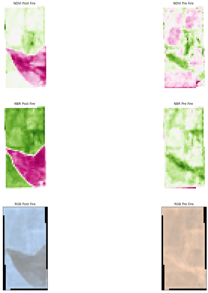
All these images clearly show the fire scar but NBR is by far the clearest as expected. I brought the exported tifs into QGIS and calculated how many acres were burned by simply drawing a polygon around the burn scar in the NBR image. In total, about 96 acres were burned. Reports said the fire started from the west and propagated east before it was put out which appears to be consistent with the burn scar.
That’s all for this analysis
We’ve successfully automated an NDVI and NBR analysis using open source python. I hope you found this helpful or at least interesting. If you have any questions please feel free to contact me.
